Handling uncertainty in the wireless channel: a Bayesian perspective

In this blog, Dr. Christo K Thomas will discuss a Bayesian approach in handling the uncertainty in the wireless channel. Currently, Christo works with Qualcomm at Espoo, Finland for 5G physical layer algorithm development (base station devices). He graduated from EURECOM, France, under the supervision of Prof. Dirk Slock, where he focused on signal processing algorithms for next-generation wireless communications with particular emphasis on hybrid or digital beamforming techniques for Massive MIMO, asymptotic analysis for Massive MIMO spectral efficiency using random matrix theory results and approximate Bayesian inference techniques. He shares a great interest in approximate Bayesian inference techniques including but not limited to belief propagation, variational Bayesian inference, expectation propagation, etc. Christo has received the best student paper award at IEEE SPS conference SPAWC2018. Their mmWave channel estimation solution won the third prize in the site-specific channel estimation challenge conducted by ITU for AI/ML in 5G competition during the year 2020.

Before joining EURECOM for Ph.D., Christo worked in the communication chip industry for around 5 years. During that time, he got employed at Broadcom communications and Intel corporation (around 2 years at both places) in Bangalore, India, where his work revolved around ASIC design for 4G LTE modem and broadband modem technology called G.FAST.

Let’s hear from Dr. Christo!

Understanding a Bayesian approach

A Bayesian approach generally starts with the formulation of a model that is adequate to describe the observed data. We also postulate a prior distribution over any unknown parameters of the model, capturing our beliefs about them before seeing the data. Once the empirical data is available, we apply Bayes’ rule to obtain the posterior distribution of these unknowns, incorporating both the prior and the data. Finding such a posterior distribution has several advantages. We can get the point estimates such as the minimum mean squared error or maximum a posteriori probability estimates and obtain higher-order statistics of these estimates. In turn, this enables better decision making and actions in many problems. In this way, Bayesian approaches can offer several advantages over non-Bayesian methods, where the model parameters are assumed to be deterministic and unknown.

What if we are ignorant of the prior information? Is it best to follow a deterministic method? In 1961, James and Stein shocked the statistical world by showing that we can obtain better estimates than the maximum likelihood estimator (MLE). For example, consider that we observe a noisy version of an unknown signal, Gaussian with non-zero mean, with the noise also being non-zero mean Gaussian. Suppose that we do not know the parameters (variance here) of x. They showed that a biased estimator (actually a scaled version of the MLE, with scale factor being proportional to an estimate of the signal variance, similar in structure to the MMSE estimator) could perform better than MLE of resulting MSE value. Even though this cannot be generalized to other settings, it was an encouraging and futuristic result for approximate inference techniques such as variational Bayesian (VB) inference.

Variational Bayesian (VB) inference

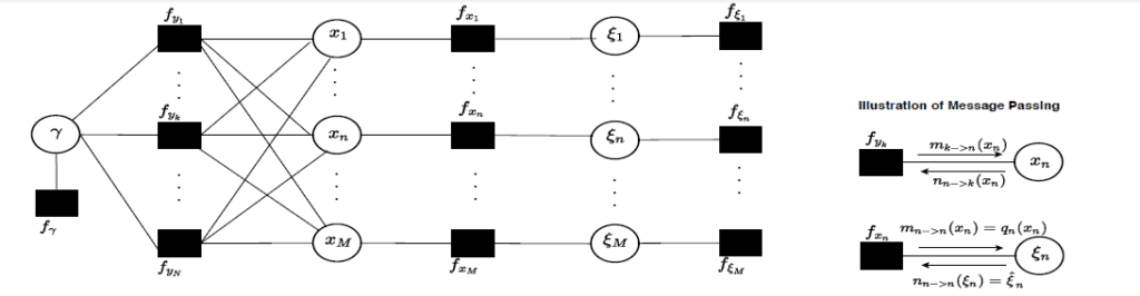
The classical deterministic estimation theory and Bayesian framework consider that the assumed data model and the actual data model (pdf) are the same. However, in practice, we prefer approximate VB inference because we may only have imperfect knowledge of the actual data model or the computational complexities associated with the computation of the exact posterior distributions. In short, variational inference schemes try to find an approximate posterior distribution by a principled approach in which we minimize the Kullback-Leibler divergence between the actual and approximate posteriors. It is essential to quantify the estimator’s performance using mismatched Cramer-Rao bounds (mCRB) in such misspecified estimation problems. The fundamental theoretical analysis of mCRB is a wide-open area of research. A popular method to solve the VB inference schemes is message passing; see for an illustration in the figure at the end.

Now, one may wonder how all this buildup to the (approximate) Bayesian inference will be of interest to the next-generation wireless technologies, 5G NR or even 6G. When we go to higher frequencies (as in mmWave band for 5G), this leads to small coherence intervals, and hence the channel tracking becomes quite challenging. We cannot afford to lose a significant chunk of the throughput for pilot signals transmission.

Extensive research in the context of 5G or beyond 5G technologies has been on how to reduce training overheads in pilot-based channel estimation. While this will be most critical in 6G, feasible solutions become extremely challenging due to the massive scale-up and connectivity demands, in particular: (i) supporting high data rates (Gbps) in high-mobility scenarios—a prime concern of operators—will require dealing with much shorter channel coherence times; (ii) ultra-low latency requirements will see shorter transmission intervals, and (iii) the number of parameters to estimate will be massively large as a consequence of the scaling (not only of antennas/APs but also of users/devices). High mobility further complicates the problem because with mobility comes issues such as faster time-variation of the channel, Doppler offsets, etc. When estimated in severe under-sampling constraints, the high-dimensional channels might render pilot-based (coherent) estimation infeasible, particularly under high-mobility or low latency requirements. Blind (non-coherent) estimation approaches—where we do not require dedicated pilot signals—stand as promising alternatives. Though significant efforts in this direction, existing methods typically require knowledge of the (high dimensional) signal covariance matrix, acquired again from a limited number of samples.

Hence the natural question is, can the existing models for channel estimation thrive under this dynamic setting? Or machine learning would be the next big thing here? Or are model-based techniques good enough? In higher frequency bands, the underlying channel is sparse in an appropriate representation, even though the channel dimensions are high. Therefore, we can represent it by a few parameters, thanks to the sparse nature or limited scattering effects at high frequency. What about the tracking? Are there good models for time-varying channels at the higher frequency bands? Probably a mix of AI and model-based techniques may be useful here in terms of developing robust estimators under model uncertainty.

Can a Bayesian approach help?

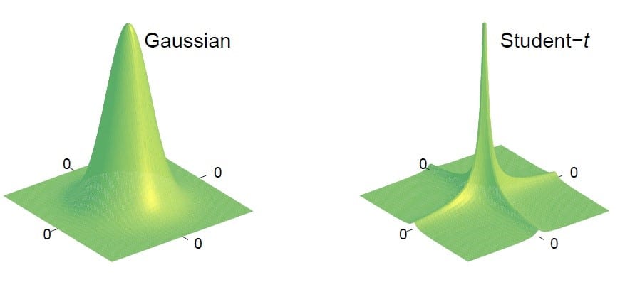
How can Bayesian inference be beneficial here? If the channel is parametric in mmWave, a joint dictionary learning and sparse signal estimation can help. The channel covariance matrix can be estimated using the AoA/AoD support information. The channel’s sparse nature can dramatically reduce the number of pilot signals required (compared to the number of antennas or subcarriers) since we only need to estimate the number of significant paths’ parametric factors. One popular algorithm which can provide substantial performance gains for such sparse channel models is sparse Bayesian learning (SBL). In sparse Bayesian learning, the underlying principle is to model the unknown sparse vectors as having a hierarchical prior distribution. For example, this follows by choosing a simple Gaussian distribution for the static or dynamic sparse states. The parameters (covariance) of this Gaussian distribution are unknown, which are modeled as some distribution, for example, a Gamma distribution. The resulting marginal distribution of the sparse vector becomes student-t, which is highly sparsifying prior.

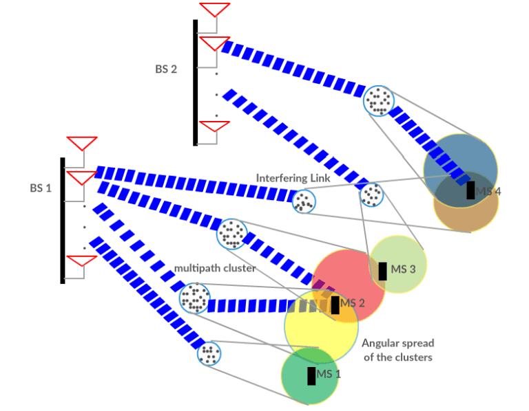
The hyperparameters here (refer Fig. 1., VB inference architecture) are learned from the pilot data using an evidence maximization procedure. SBL can be extended to the scenarios when the underlying sparse signals are structured or block sparse as in stochastic geometry-based mmWave channel models. However, the original SBL algorithm can become computationally expensive due to its iterative nature, especially in high dimensional settings (massive MIMO) or when we need to learn complicated prior covariance matrices. There are several ultra-fast versions of SBL that are available in the literature. Alternatively, an efficient strategy could be to unfold the iterations (Expectation-Maximization (EM) ) in hyperparameter learning into a deep neural network (DNN) if we have enough data available, which helps us to learn the scattering geometry between the users to the base station. We expect that many such low complexities and high-performance solutions will be available beyond 5G/6G shortly.

Acknowledgments: The author is extremely grateful to his supervisor, Prof. Dirk Slock, at EURECOM, France, for introducing the approximate Bayesian inference during his Ph.D. The author would also like to thank Prof. Chandra R Murthy, IISc, Bangalore, India, for providing useful feedback for this write-up.

**Statements and opinions given in this blog are the expressions of the contributor(s). Responsibility for the content of published articles rests upon the contributor(s), not on the IEEE Communication Society or the IEEE Communications Society Young Professionals.